A Crashcourse to FEM

Given the limitations in space and time, this is a brief introduction to the Finite Element Method (FEM). Interested readers are referred to the classic textbook by Belytschko and Fish [12], the excellent lecture notes by Dennis Kochmann (https://mm.ethz.ch/education/lecture-notes.html), and the textbook by Peter Wriggers [13] for advanced topics. This section outlines the basic “recipe” to discretize a physical problem described by a partial differential equation (PDE) using FEM which is commonly done the following the steps:

• derive weak form

• if PDE nonlinear: linearize

• approximate weak form

In this section we will restrict ourselves to examples of linear problems and only hint or show final results for nonlinear problems.

From Strong to Weak Form

Most physical problems can be written as PDEs based on a conservation law or other physical insights. Classical examples are the Poisson equation

\[\nabla \cdot (\boldsymbol{\Lambda} \nabla \phi) = f\]

governing heat conduction or diffusion with scalar variable \(\phi\) (temperature, concentration, etc.) and property tensor \(\boldsymbol{\Lambda}\), the continuity equation

\[\frac{\partial \rho}{\partial t} + \nabla \cdot (\rho \boldsymbol{v}) = 0\]

describing conservation of mass (density \(\rho\), time \(t\) and velocity field \(\boldsymbol{v}\) and the Cauchy momentum balance

\[\rho \ddot{\boldsymbol{u}} = \nabla \cdot \boldsymbol{\sigma} + \boldsymbol{b}\]

representing conservation of linear momentum with the Cauchy stress tensor \(\boldsymbol{\sigma}\), body force \(\boldsymbol{b}\) and displacement \(\boldsymbol{u}\) . Combined with a constitutive law (e.g. Hooke’s law \(\boldsymbol{\sigma} = \boldsymbol{C} : \boldsymbol{\epsilon}\) with stiffness tensor \(\boldsymbol{C}\) and engineering/incremental strain tensor \(\boldsymbol{\epsilon}=\frac{1}{2}\left(\nabla \boldsymbol{u} + \nabla \boldsymbol{u}^T \right)\)), this gives the mechanical response of a solid. For small deformations, inserting Hooke’s law yields the Navier–Lamé equations

\[\rho \ddot{\boldsymbol{u}} = \nabla \cdot \left( \boldsymbol{C} : \boldsymbol{\epsilon} \right) + \boldsymbol{b},\]

and for Newtonian fluids the Navier–Stokes equations

\[\rho \left( \frac{\partial \boldsymbol{v}}{\partial t} + \boldsymbol{v}\cdot\nabla\boldsymbol{v} \right) = -\nabla p + \mu \nabla^2 \boldsymbol{v} + \rho \boldsymbol{b}.\]

All of these equations are expressed in terms of their derivatives i. e. differential form which we call the strong form. We introduce a generic PDE for brevity as

\[\mathcal{L}(u) = f \quad \text{in } \Omega,\]

where the linear differential operator \(\mathcal{L}\) represents all terms with derivatives involving the unknown field \(u\) (e. g. for linear elasticity \(\nabla \cdot \left( \boldsymbol{C} : \boldsymbol{\epsilon} \right)\)), \(f\) represents any inhomogeneous terms often called source/sink terms and \(\Omega\) the simulation domain. In terms of boundary conditions, we only concern ourselves in this article with Dirichlet boundary conditions that fix the state variable to specific values on a part of the boundary \(\Gamma_D\)

\[u = u_{D} \quad \text{on } \Gamma_{D}\]

and von Neumann boundary conditions that prescribe the value of the first normal derivative(s) across the boundary plane with normal \(\boldsymbol{n}\) on a part of the boundary \(\Gamma_N\) to value \(\partial u_{N}\)

\[\nabla u^T \boldsymbol{n} = \partial u_{N} \quad \text{on } \Gamma_{N}\]

We assume that the total boundary \(\Gamma\) consists of Dirichlet and Neumann boundaries, i. e. \(\Gamma = \Gamma_D \cup Gamma_N\). In solid mechanics, Dirichlet boundary conditions correspond to displacement boundary conditions while in heat conduction or diffusion they correspond to temperature/concentration boundary conditions. Von Neumann boundary conditions are often formulated differently, as in real cases often the gradient of the state variable \(u\) is unavailable, but instead the flux is measured, so the above equation is simply rescaled by some material constants

\[\left(\boldsymbol{\Lambda} \nabla u\right)^T \boldsymbol{n} = q_{N} \quad \text{on } \Gamma_{N}\]

which however does not change the nature of the boundary condition: it is still a boundary condition in terms of the first order derivatives.

To arrive at the weak form, we multiply the strong form and the boundary conditions by a weight function \(w\) or often also called test function and integrate over the domain \(\Omega\), so we end up with

\[\begin{split}\int_\Omega w \, (\mathcal{L}(u) - f) \, dV = 0 \\ \int_{\Gamma_{N}} w ( \boldsymbol{\Lambda} \nabla u)^T \boldsymbol{n} dA = u_{N}.\end{split}\]

The weak form is fully equivalent to the strong form only if \(u\) and \(w\) satisfy some conditions. Among these conditions are \(w!=0\) and that the weak form must hold for abitrary (!) \(w\) as then the residual \(r\)

\[r=\int_\Omega w \, (\mathcal{L}(u) - f) \, dV \]

vanishes everywhere, which corresponds to the solution of the strong form. The weight function \(w\) is also useful from a numerical perspective as we will later see, it allows to use less smooth, i. e. cheaper approximations and it naturally introduces boundary terms for Neumann boundary conditions. Furthermore, from a numerical perspective, it is often convenient to work with integrals as they can be approximated cheaply.

Example: Weak form of Poisson equation

In this paragraph we will write down the weak form for the Poisson equation which guides an abundant number of physical phenomena like temperature conduction, diffusion, gravity, electrostatics, etc. pp. For sake of brevity, we focus on time-independent (stationary) heat conduction. We start with the weak form via standard procedure i) multiply PDE and boundary conditions by \(w\) ii) integrate over domain \(\Omega\):

\[\begin{split}\int_\Omega w \nabla \cdot (\boldsymbol{\Lambda} \nabla \phi) dV = \int_\Omega w f dV \\ \int_{\Gamma_{N}} w\left(\boldsymbol{\Lambda} \nabla \phi\right)^T \boldsymbol{n} dA\end{split}\]

Technically one can stop now as this is a correct weak from, but we want to reduce the highest order derivative as much as we can as in FEM this means we can approximate it cheaper. We split weak form into left hand side and right hand side and consider the “problematic” left hand side

\[\int_\Omega w \nabla \cdot (\boldsymbol{\Lambda} \nabla \phi) dV\]

to simplify it further. We remember the chain rule for a general vector \(\boldsymbol{v}\) and the scalar function \(w\)

\[\nabla \cdot (w\boldsymbol{v}) = w\nabla \cdot \boldsymbol{v} + \nabla w \cdot \boldsymbol{v}\]

which we rewrite to

\[w\nabla \boldsymbol{v} = \nabla w \cdot \boldsymbol{v} - \nabla \cdot (w\boldsymbol{v})\]

We then insert \(\boldsymbol{v}=\nabla \phi\) and rewrite the left hand side to

\[\int_\Omega w \nabla \cdot (\boldsymbol{\Lambda} \nabla \phi) dV = \int_\Omega \nabla w \cdot \boldsymbol{\Lambda} \nabla \phi dV - \int_\Omega \nabla \cdot w\left(\boldsymbol{\Lambda} \nabla \phi\right) dV\]

If we inspect this closer, we recognize that the second term on the right hand side is the volume integral of the divergence of the flow \(\boldsymbol{\Lambda} \nabla \phi\) scaled by \(w\). In simple words, this integral describes how much of \(w \boldsymbol{\Lambda} \nabla \phi \) is being produced or lost within the volume. Instead of measuring what happens inside, we can equivalently measure how much of \(w \boldsymbol{\Lambda} \nabla \phi \) flows in or out through the surface enclosing it which is what the divergence theorem expresses

\[\int_{\Omega} \nabla \cdot \boldsymbol{v} dV = \int_{\Gamma} \boldsymbol{v} \cdot \boldsymbol{n} dA \]

which we can use to simplify the second part to

\[\int_\Omega \nabla \cdot w\left(\boldsymbol{\Lambda} \nabla \phi\right) dV = \int_{\Gamma_{N}} w\left(\boldsymbol{\Lambda} \nabla \phi\right)^T \boldsymbol{n} dA \]

This boundary flux conveniently represent the von Neumann boundary conditions, so they appear naturally in the weak form which is why they are often referred to as natural boundary conditions in FEM terminology. We write down the full weak form in its simplified form

\[\int_\Omega \nabla w \cdot \boldsymbol{\Lambda} \nabla \phi dV - \int_{\Gamma_{N}} w\left(\boldsymbol{\Lambda} \nabla \phi\right)^T \boldsymbol{n} dA = \int_\Omega w f dV.\]

Since we want to solve for \(phi\) while both the von Neumann boundary conditions and the function \(f\) are given, we move the von Neumann terms to the right hand side such that we have cleanly divided the weak form in the terms we seek to solve/invert and the terms that are part of the problem statement, i. e. the boundary conditions:

\[\int_\Omega \nabla w \cdot \boldsymbol{\Lambda} \nabla \phi dV = \int_\Omega w f dV + \int_{\Gamma_{N}} w\left(\boldsymbol{\Lambda} \nabla \phi\right)^T \boldsymbol{n} dA.\]

We now demand \(\phi\) to fulfill the Dirichlet boundary conditions on \(\Gamma_D\) by \(\phi=\phi_D\) and \(w=0\). Why \(w=0\)? Technically

Discretization of Weak Form

Since the weak form is an integral, we can now slowly see how elements as subdivisions of the simulation domain emerge: integrals are additive, meaning an integral over interval \(a\) to \(c\) can be split into sub-intervals \(a\) to \(b\) and \(b\) to \(c\)

\[\int_a^c ... dx = \int_a^b ... dx + \int_b^c ... dx\]

so we can re-write the weak form to

\[\sum_{e=1}^{N_{e}}\int_{\Omega_e} \left(\nabla w\right)^T \boldsymbol{\Lambda} \nabla \phi dV_{\Omega_e} = \sum_{e=1}^{N_{e}} \int_{\Omega_e} w f dV_e + \int_{\Gamma_{N,e}} w\left(\boldsymbol{\Lambda} \nabla \phi\right)^T \boldsymbol{n} dA_e.\]

where the index \(e\) is the element index. So in other words an element is just a sub-interval/area/volume of the entire domain. This step is purely geometric and does not yet introduce any approximation as it just rewrites the weak form as a sum of element-wise contributions that via simple summation assemble the global problem. We now move on, how to approximate these integrals to arrive at a continuous, smooth solution.

Shape Functions and Interpolation

After splitting the domain into elements, a few things need to be kept in mind: i) we need to approximate the unknown field \(u\) inside each element to solve the local element integrals. ii) the values of \(u\) at the element borders should match for the smoothness and continuity required by the PDE. The natural choice for these requirements are piecewise defined polynomials, i. e. splines, as they only require nodal values at the border between elements for interpolation, due to their local polynomial nature are easy to integrate (even high school students could do it) and offer flexibel smoothness/continuity via the choice of order. As a rule of thumb, it is preferable to choose the lowest order of spline that is sufficient to solve the PDE at hand. Having chosen splines an interpolation, we can now express both the unknown field \(u\) and the test function \(w\) in terms of these local basis functions. This turns the continuous fields into finite sets of nodal values, which can then be used directly in the weak form on each element.

Interpolation with Lagrange Polynomials

For simplicity, we start with 1D and assume we know the values of the function \(\phi\) we seek to interpolate at \(n\) positions with value \(\phi_i\) at point with coordinate \(x_i\). In FEM we call these points nodes. We require that i) the interpolation function \(\phi_e(x)\) passes exactly through the points \(\phi_i=\phi_e(x_i)\) ii) the interpolation function \(\phi_e(x)\) should be simple and fast to evaluate. iii) the interpolation function \(\phi_e(x)\) is flexible to fulfill smoothness requirements for the PDE at hand and ideally tuneable to the order of PDE.

For requirement ii) we write as linear combination of functions \(N_i(x)\) associated with each point \(i\)

\[\phi_e(x) = \sum_{i=1}^{n} N_{i}\left(x;x_i\right)\phi_{i}.\]

Now if we demand \(N_i(x_i)=1\) and \(N_i(x_{j \neq i)=0\), then requirement i) is satisified which is referred to as the delta-property. We have not yet specified the nature of the generic functions \(N_i(x)\). A simple class of functions with tuneable smoothness are polynomials. A polynomial fulfilling \(N_i(x_{j \neq i)=0\) is

\[\prod_{j=1,j \neq i}^{n} (x-x_j),\]

which is modified to fulfill \(N_i(x_i)=1\) by adding the denominator \(x_i-x_j\), therefore the final interpolating polynomials read as

\[N_i(x)= \prod_{j=1,j \neq i}^{n} \frac{x-x_j}{x_i-x_j}.\]

These are called Lagrange polynomials and are the most frequently used interpolation functions in FEM.

The element matrix for the Poisson equation

We restrict ourselves to the standard Galerkin finite element method where both \(w\) and \(u\) are approximated by the same functions, i. e. are interpolated in the same function space. We therefore refer to them as shape functions. In general, \(u\) and \(w\) inside element \(e\) are approximated as

\[u_e(x) = \sum_{j=1}^{n} N_{j}\left(x;x_j\right)u_{j}\]

\[w_e(x) = \sum_{j=1}^{n} N_{j}\left(x;x_j\right)w_{j}\]

or more commonly in vector format as

\[u_e(x) = \boldsymbol{N}^T \boldsymbol{u}_n\]

\[w_e(x) = \boldsymbol{N}^T \boldsymbol{w}_n.\]

where \(n\) is the number of nodes in the element, \(u_{i},w_{i}\) are the value of \(u,w\) at the nodes and \(N_{i}\) the shape function associated with node \(i\). Generally these shape functions constitute of polynomial functions in terms of space and take the value \(1\) at \(x_i\) and the value \(0\) at nodes \(i \neq j\).

We now take the weak form for a single element

\[\int_{\Omega_e} \left(\nabla w_e\right)^T \boldsymbol{\Lambda} \nabla \phi_e dV_{\Omega_e} = \int_{\Omega_e} w_e f_e dV_e + \int_{\Gamma_{N,e}} \left(w_e \boldsymbol{\Lambda} \nabla \phi_e\right)^T \boldsymbol{n} dA_e.\]

and insert our approximation

\[\boldsymbol{w}_{n}^T \int_{\Omega_e} \left(\nabla \boldsymbol{N} \right)^T \boldsymbol{\Lambda} \nabla \boldsymbol{N}^T dV_{\Omega_i} \boldsymbol{\phi}_n = \boldsymbol{w}_e^T \left[ \int_{\Omega_e} \boldsymbol{N} f dV_e + \int_{\Gamma_{N,e}} \boldsymbol{N} \left( \boldsymbol{\Lambda} \nabla \phi\right)^T \boldsymbol{n} dA_e \right].\]

After some careful consideration, we recognize the left hand side as a linear system

\[\boldsymbol{w}_n^T \int_{\Omega_e} \boldsymbol{A} \boldsymbol{\phi}_n = \boldsymbol{w}_n^T \int_{\Omega_e} \left(\nabla \boldsymbol{N} \right)^T \boldsymbol{\Lambda} \nabla \boldsymbol{N}^T dV_{\Omega_i} \boldsymbol{\phi}_n.\]

\(\boldsymbol{w}_n\) must not matter as the requirement for the weak form to deliver a solution to the original PDE was that \(w\) must be arbitrary. This reduces the expression further to

\[\boldsymbol{K}_e \boldsymbol{\phi}_n = \int_{\Omega_e} \left(\nabla \boldsymbol{N} \right)^T \boldsymbol{\Lambda} \nabla \boldsymbol{N}^T dV_{\Omega_i} \boldsymbol{\phi}_n.\]

We call \(\boldsymbol{K}_e\) the element conductivity matrix or sometimes due to its analogy to linear elasticity the element stiffness matrix. We now need to insert this element matrix in to the wider context of the entire problem as an indivual element only represents a small section of the entire problem.

Assembly of Global Linear Problem

We recall that we receive the local element matrix from the additivity property of integrals, meaning an integral over interval \(a\) to \(c\) can be split into sub-intervals \(a\) to \(b\) and \(b\) to \(c\)

\[\int_a^c ... dx = \int_a^b ... dx + \int_b^c ... dx.\]

therefore we can write a global system matrix \(\boldsymbol{K}\) as the sum over the local element matrices

\[\boldsymbol{K}= \sum_{e=1}^{N_e} \boldsymbol{K}_e.\]

to receive the global problem

\[\boldsymbol{K}\boldsymbol{\phi}= \boldsymbol{f}.\]

To construct \(\boldsymbol{K}\), we must be able to map the nodal values \(\phi_n\) of a local element to the global degrees of freedom (dofs) \(\boldsymbol{\phi}\) which is just a matter of bookkeeping. We define a local node ordering e. g. for a 4-node bilinear quad (Q4) element

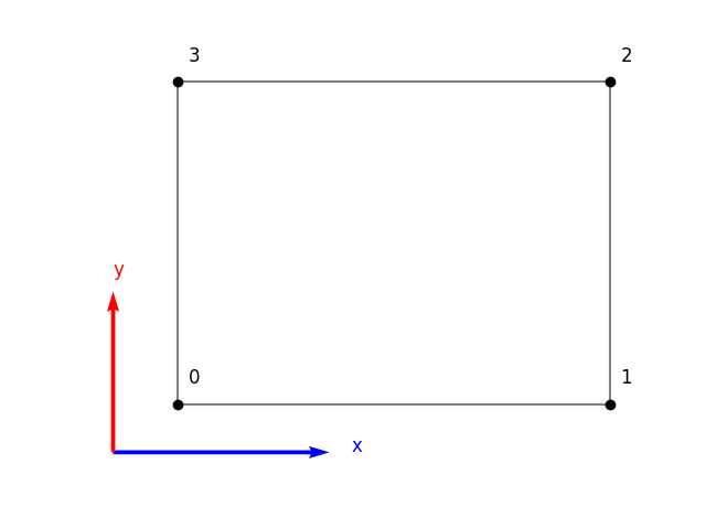
and the global node numbering (arabic numbers for node numbers, roman for elements)

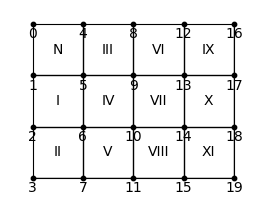
We then define the element-degree-of-freedom matrix (edofMat) which contains the dofs associated with each element in sequence of the local ordering but with their global indices. Let’s look at the entry of the first element (element index ‘N’) in the edofMat where we write first the global index of the bottom left node, then the bottom right node, the upper right and last the upper left index (we use C-indexing, so indices start from zero):

\[1 \quad 5 \quad 4 \quad 0\]

The complete edofMat then is

\[ \begin{align}\begin{aligned}1 \quad 5 \quad 4 \quad 0\\2 \quad 6 \quad 5 \quad 1\\3 \quad 7 \quad 6 \quad 2\\5 \quad 9 \quad 8 \quad 4\\6 \quad 10 \quad 9 \quad 5\\7 \quad 11 \quad 10 \quad 6\\9 \quad 13 \quad 12 \quad 8\\10 \quad 14 \quad 13 \quad 9\\11 \quad 15 \quad 14 \quad 10\\13 \quad 17 \quad 16 \quad 12\\14 \quad 18 \quad 17 \quad 13\\15 \quad 19 \quad 18 \quad 14\end{aligned}\end{align} \]

So if we set up \(\boldsymbol{K}\), we start with the first element and its element matrix \(\boldsymbol{K}^e\). We update the diagonal (\(+=\) means adding on the already existing value)

\[ \begin{align}\begin{aligned}K_{1,1} += K_{0,0}^{e}\\K_{5,5} += K_{1,1}^{e}\\K_{4,4} += K_{2,2}^{e}\\K_{0,0} += K_{3,3}^{e}\end{aligned}\end{align} \]

For the off-diagonals, the same procedure applies which we demonstrate for the first row of \(\boldsymbol{K}_e\)

\[ \begin{align}\begin{aligned}K_{1,5} += K_{0,1}^{e}\\K_{1,4} += K_{0,2}^{e}\\K_{1,0} += K_{0,3}^{e}\end{aligned}\end{align} \]

For the other rows the method is exactly the same. We repeat this for every element which yields the final global linear system \(\boldsymbol{K}\).

Numerical Integration

Since the shape functions are polynomials within each element, evaluating the integrals for each entry of \(K_e\) is analytically possible, but especially in higher dimensions and with higher-order shape functions is error-prone. Luckily, numerical integration via quadrature automates this task efficiently with the most prominent case of Gauss quadrature. We consider an integral of an arbitrary function \(f\) defined over the interval \([-1,1]\) and re-write the integral as a weighted sum of the function values at a number \(n_q\) of specific points referred to as integration points \(\xi_q\), Gauss points or quadrature points, with weights \(\omega_q\)

\[\int_{-1}^{1}f(\xi)\,d\xi\approx\sum_{q=1}^{n_q}\omega_q\,f(\xi_q).\]

The weights \(\omega_q\) are pre-computed to guarantee exact integration with \(n_q\) points for all polynomials up to order \(2n_q-1\) within the interval \(\xi \in [-1,1]\). Given our polynomial shape functions, to use this efficient integration method, the integral over the element domain \(\Omega_e\)​ is mapped to the reference frame \(\xi \in [-1,1]\) and all computations are carried out there using the chosen quadrature rule. While in 1D this mapping is a simple rescaling, in higher dimensions this process requires a bit more care and does not guarantee exact integration anymore as the mapped integral will not be polynomial, which is the topic of the next subsection.

Isoparametric Map

In higher dimensions, for efficient integrations and shape-function evaluations we map to a simple reference element and then map the results to the actual (possibly distorted), physical element in the global coordinate system. We notate the coordinates in the reference frame by greek letters \(\xi\),\(\eta\),\(\zeta\) or collectively as \(\boldsymbol{\xi}\). We then approximate the map \(\boldsymbol{\psi}_e(\xi,\eta,\zeta)\) from coordinates in the reference frame to the physical coordinates of the actual element by shape functions and nodal coordinates \(\boldsymbol{x}_n\) with the same approach earlier used for the ansatz for the state variable and the weight function:

\[\begin{split}x_e(\xi,\eta,\zeta) = \boldsymbol{N}(\xi,\eta,\zeta)^T \boldsymbol{x}_n \\ y_e(\xi,\eta,\zeta) = \boldsymbol{N}(\xi,\eta,\zeta)^T \boldsymbol{y}_n \\ z_e(\xi,\eta,\zeta) = \boldsymbol{N}(\xi,\eta,\zeta)^T \boldsymbol{z}_n\end{split}\]

In most FEM problems we also have to evaluate gradients like in our example of the Poisson equation. As we want to carry out the calculations in the reference frame, we need to consider how to evaluate the gradients in the reference frame. We notice in 1D, as a special case to guide our intuition, that if we consider the gradient of a function in the reference frame

\[\frac{\partial f}{\partial \xi} = \frac{\partial f}{\partial \psi_e} \frac{\partial \psi_e}{\partial \xi} \]

we can reformulate the approximate gradient \(\frac{\partial f}{\partial x_e}\) by

\[\frac{\partial f}{\partial x_e} = \frac{\partial f}{\partial \xi} \left(\frac{\partial \psi_e}{\partial \xi}\right)^{-1}\]

which is purely formulated in terms of the node coordinates \(\boldsymbol{x}_n\) and the shape functions which are formulated in reference space. With that in mind we consider

-collect nodal coordinates in matrix \(\boldsymbol{X}_n\) with every column for a spatial dimension -write nodal coordinates therefor in vector notation

\[\tilde{\boldsymbol{x}}_e(\boldsymbol(x)) = \boldsymbol{N}^T \boldsymbol{X}_n \]

-show the implicit