Introduction to Topology Optimization
In this article we introduce the basic concepts behind topology optimization (TO). We will implicitly assume that the finite element method (FEM) is the underlying discretization technique, but TO is a general technique that is not tied to any specific numerical technique. Loosely speaking in TO we set out to find the optimal design parameters \(\boldsymbol{x}\) for a given objective function \(C(\boldsymbol{x})\), a set of equality as well as inequality constraints on the design \(\boldsymbol{g}(\boldsymbol{x}),\boldsymbol{h}(\boldsymbol{x})\) and a set of discretized physical problems \(\boldsymbol{K}(\boldsymbol{x}) \boldsymbol{u} = \boldsymbol{f}\) with associated boundary conditions:
Common choices here are material volume constraints reflecting economic/monetary constraints or stress constraints to guarantee structural stability. The question arises now, what are the design parameters \(\boldsymbol{x}\) ? A straightforward, intuitive approach would be to switch each finite element in the design between two states: either solid or void which is the same as deleting the element from the FEM. This results in a discrete optimization problem where \(x_e \in \{0,1\}\) for each element \(e\) which leads to a combinatorial explosion in the number of design possibilities and is also known to suffer from severe numerical problems (convergence, stability, efficiency, …). Density-based TO on the other hand employs a continuous relaxation of the concept of solid/void by introducing artificial relative material densities \(x_e \in [0, 1]\) for each element, allowing for a continuous interpolation between a void state (\(x = 0\)) and a fully solid state (\(x = 1\)). This enables the use of constrained optimizers like the Method of Moving Asymptotes (MMA) [1] and its globally convergent modification (GCMMA)[2] which are known to converge fast and reliably to optimal designs. A common interpolation scheme is the modfied Solid Isotropic Material with Penalization (SIMP) [3] method in which the interpolation of material property \(A(x_e)\) takes the form:
Here, \(A_0\) denotes the property of the full material, \(A_{\min}\) is a small positive number used to avoid singularity in the stiffness matrix (typically \(10^{-9} A_0\)), and \(k > 1\) is a penalization exponent. It is important to emphasize that this interpolation is not arbitrary. It must obey physical bounds—such as the Hashin–Shtrikman limits—to ensure that the resulting material behavior remains physically meaningful. From a practical standpoint, the interpolation should be constructed such that intermediate densities (i.e., gray areas) do not influence the physical problem significantly, since this forces the optimizer to avoid choosing gray values, as they require significant “investment” in density to meaningfully alter the objective function and constraints. This not only improves numerical stability but also yields designs that are more amenable to manufacturing. After the optimization, the continuous densities are thresholded to a “black-and-white” designs of discrete densities 0/1. If volume constraints have been applied, the thresholding must obviously take the constraint into account.
We now proceed naively and try to find the classical result for the stiffness maximization of the MBB beam: we calculate the gradients (in TO typically called sensitivities) necessary for the optimization \(\nabla_{\boldsymbol{x}} C = 0\) via adjoint analysis (Adjoint Analysis) and use a constrained optimizer (e. g. MMA) which yields a strange design with artifacts commonly known as checkerboard patterns.
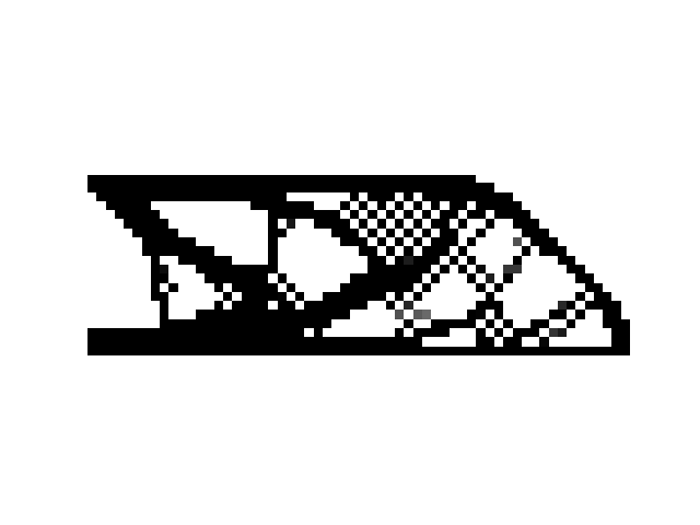
These patterns arise because the optimizer abuses short comings of low-order elements to model the mechanical problem. An (expensive) solution would be to employ higher order elements, but that just reveals another problem: the designs show mesh dependence and even minor changes in discretization will cause the final design to change, i. e. the results of TO are mesh dependent. The first ad-hoc countermeasure was to apply a smoothing filter (identical to the filter used in image processing) with radius \(r\) to the sensitivities as this prevents the concentration of gradients therefor mitigating the appearance of checkerboards[4] and also yields the same results if the mesh is refined further as the filter radius \(r\) determines the smallest length scale of the design.
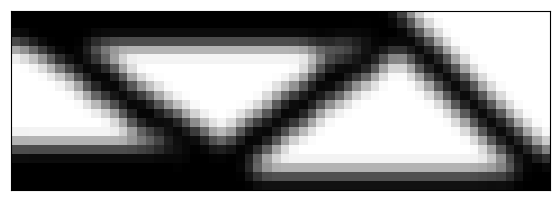
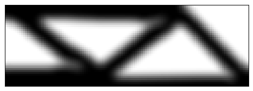
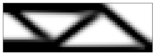
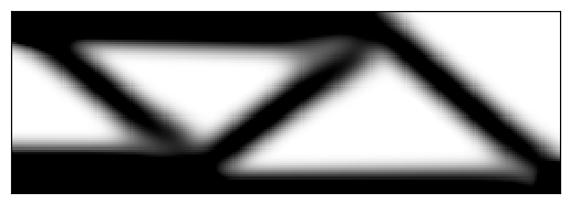
Figure: Convergence demonstration of topology optimization for different mesh refinements with constant filter radius. Top row density filter bottom row sensitivity filter.
|
|
|
|---|---|---|
|
|
|


While intuitive and effective, this changes the original objective function \(C\). For the stiffness maximization in linear (local) elasticity, it can be shown that sensitivity filtering changes the objective function to stiffness maximization in nonlocal elasticity[5]. A solution that leaves the original objective function untouched is the smoothing of the design densities and guarantees well-posedness and mesh-independence[6]. This operation can be written via a convolution integral
where \(H(r,s)\) is the convolution kernel (in most cases is a linear hat function) and \(\Omega\) the optimization domain. At this point we have to clearly distinguish between the design variables \(\boldsymbol{x}\) and the filtered variables \(\boldsymbol{x}_p\): \(\boldsymbol{x}_p\) are used in the material interpolation and thus are called “physical” densities as they directly manipulate the physical properties while \(\boldsymbol{x}\) describe the design. To update the design \(\boldsymbol{x}\) has to be changed, but adjoint analysis yields only \(\frac{\partial C}{\partial x_{p}}\), so the chain rule has to be used to recover \(\frac{\partial C}{\partial x}\):
By now, a first preliminary TO workflow in pseudo Python code can be stated:
# initialize design and simulation settings
x = initialize_designdensities()
filters = initialize_filters()
initialize_fem()
x_filtered = filter(x)

# start design iteration loop
for i in range(max_designiterations):

    # interpolate material properties
    props_scaled = interpolate_properties(x_filtered,props)

    # solve phys. problem (here FEM)
    state_variables = solve_FE(props_scaled)

    # compute objective function and return right hand side of adjoint problem
    obj,adj_problem_rhs = compute_obj(state_variables,x,x_filtered,...)


    # calculate sensitivities with respect to physical densities
    dobj = solve_adjoint_prob_obj(state_variables,adj_problem_rhs)

    # repeat the same for constraints
    constrs = np.zeros(number_of_constraints)
    constrs = np.zeros((x_filtered.shape[0],number_of_constraints))
    i = 0
    for constraint in constraints:
        constr[i],adj_problem_rhs = constraint(state_variables,x,x_filtered,...)
        dconstrs[:,i] = solve_adjoint_prob_constraints(state_variables,adj_problem_rhs)

    # recover sensitivities with respect to design variables
    dobj = filters_dx(dobj)
    dconstrs = filters_dx(dconstrs)

    # apply optimzer to update design variables
    x = constrained_optimizer(x, dobj, dconstrs)

    # filter design variables
    x_filtered = filters(x)

    # check convergence criteria
    check = check_convergence()
    if check:
       break
#
export_final_design()
This is also the workflow that runs under hood of the topology_optimization.py.
Closing Remarks
In many cases, simple smoothing is not enough to get rid of numerical artifacts and different filters or combinations thereof must be used. Among many other things, filtering can be used to create near black and white design via smooth Haeviside filters or to guarantee a manufactureable design [7]. So far, only density-based TO with the modified SIMP interpolation has been presented, but other interpolation schemes like RAMP exist and are required e. g. for multimaterial oprimization.
Recommended References
For further reading regarding TO, the following references are recommended:
review article from 2013 [8]: one of the first places to start if one is new to the topic and gives a good overview over different approaches to TO
an educational article with associated Matlab code [9]: read the paper and compare with the “translation” to Python in the monolithic_codes directory
the standard textbook by Sigmund and Bendsoe[10]: still the gold standard in my opinion, but sometimes expects considerable knowledge about finite elements and optimization. Preferably read the two previous articles before starting this book.
more recent overview with special focus on TO for manufactureable designs [11]: the first third is one of the most complete overview of TO in recent years, the latter two thirds do not deal with TO
For people unfamiliar with FEM or in need of refreshing the following books and lectures have been useful to me:
classic textbook [12]: the first five chapters are in my opinion a must for people new to FEM
lecture material by Dennis Kochmann for his course “Introduction to Finite Element Analysis” https://mm.ethz.ch/education/lecture-notes.html : excellently written, easy to understand and very useful when trying to understand the FE implementation in this code
advanced textbook by Peter Wriggers [13]: covers anything that the previous two have not covered and for me the first place to look for problems beyond the basics.